Problem set #4 PHY256
Problem 1. Integrating a 1 dimensional equation of motion (ODE) and rescaling
We will use the function odeint (or you can use solve_ivp) from scipy.integrate to integrate an ordinary differential equation (ODE) that we can solve analytically. This will let us check that it works. ivp means initial value problem.
A dynamical equation decribing a decay rate (the amount of $y$ drops by an amount that depends on the amount of $y$ around and with a rate set by parameter $a$ $$ \frac{dy}{dt} = - ay $$ with initial value $$y(0) = y_0$$ has exponentially decaying solution $$y(t) = y_0 e^{-at}$$
An example of a system that obeys this equation is the decay of a radioactive element and $a$ is proportional to the half-life of the element. Another example might be the decaying voltage in an RC circuit.
For a tutorial on how to use odeint or solve_ivp see
https://docs.scipy.org/doc/scipy/reference/generated/scipy.integrate.odeint.html
http://docs.scipy.org/doc/scipy/reference/tutorial/integrate.html
In the example below I show that the integrated solution lies on top of the analytically predicted one.
# example, integrating with odeint an exponential decaying function
%matplotlib inline
import numpy as np
from scipy.integrate import odeint
import matplotlib.pyplot as plt

#initial condition
y0 = 1.5
a = 0.5  # global variable !!!

# Set up time grid for integration
tmax=10.0;
dt = 0.2;
tt = np.arange(0,tmax,dt);  # the time vector
# this is a list of times.  odeint will return solutions at these times

# our ordinary differential equation
def func(y,t):  # equation for motion! this is dy/dt
    return -a*y

# our analytical solution given initial value y0 and time t
def ysol_func(y0,t):
    return y0*np.exp(-a*t)

# solve the ordinary differential equation
yy=odeint(func,y0,tt)  # func is our function, y0 is initial condition,
# tt a time vector
# yy is now a vector yy values computed by integrating the equation
# we will have a y value at each time in the vector yy

# plot the predicted analytical solution on top of the integrated solution
ysol = ysol_func(y0,tt)   # vector of y values predicted
plt.plot(tt,yy,'ro',label="integrated")  # plot the ingegrated thing as points
plt.plot(tt,ysol,'b-',label="predicted")  # plot the analytical solution as a line
plt.xlabel("time t",fontsize=22)  # make nice labels!
plt.ylabel("y",fontsize=22)
plt.legend(loc='best',frameon=False,fontsize=15)  # legend

# how well did the integration do?
print ('error ', yy[-1] - ysol[-1]);  # difference at the end

My predicted function lies on top of my integrated function!
# example using solve_ivp which has completely different formats for everything!
# !#&#$@#$@#

from scipy.integrate import solve_ivp

# our ordinary differential equation
def func2(t,y):  # equation for motion! this is dy/dt, reversing order
    return -a*y

# our analytical solution given initial value y0 and time t, reversing order
def ysol_func2(t,y0):
    return y0*np.exp(-a*t)

tmax = np.max(tt)
sol=solve_ivp(func2,[0,tmax],[y0],t_eval=tt,atol=1e-10) #  arguments are not in the same order
# analytical solution
ysol = ysol_func2(tt,y0)
plt.plot(sol.t,sol.y[0],'ro')  # plot the ingegrated thing
plt.plot(tt,ysol,'b-')  # plot the analytical solution
plt.xlabel("time",fontsize=20)
plt.ylabel("y",fontsize=20)

#How well did it do?
print('error ' , ysol[-1]- sol.y[0,-1])

My predicted function lies on top of my integrated function!
Problem 1
Modify one of the example codes above to numerically integrate the ordinary differential equation $$ \frac{dy}{dt} = 1+y^2 $$
You will probably need to keep $t < 2$ to keep the solution from going to infinity.Find the analytical solution to this ordinary differential equation. The integral $\int \frac{dy}{y^2 +1} $ can be computed without much effort using https://www.wolframalpha.com/ or you can look it up from a list of integrals or you can use variable subsitution to find the integral. Your analytical solution will depend on your initial condition or $y_0 = y(t=0)$.
Compare a numerically integrated solution to one you find analytically. Plot one on top of the other! See if you can improve the accuracy of your integration by adjusting the parameter rtol or atol.
error = rtol * abs(y) + atolrtol is a relative tolerance in terms of fraction of $y$.
atol is an absolute tolerance.
Here error is a local error so the accumulated error can exceed this.
- Show that by rescaling the y coordinate and time, any equation in the form $$ \frac{dz}{d\tau} = a + b z^2$$ with constants nonzero $a,b$ can be rewritten like the previous version. In other words show that you can find constants $\alpha, \beta$ such that $z = \alpha y$ and $\tau = \beta t$ giving $$ \frac{d{ y}}{dt} = 1 + y^2 $$ Give expressions for $\alpha,\beta $ in terms of $a,b$.
Why?
When doing numerical work it is a good idea think of ways to test your code.
Comparing a known solution to an integrated one is one way to test the accuracy of a code.
Often we solve problems in numerical units. The numerical output is then converted to physical units. The last part of the problem illustrates this concept.
Problem 2. A Qubit class object
- Write a python class that stores the state of a qubit. A state for the qubit looks like $$| \psi \rangle = a | 0 \rangle + b| 1\rangle$$ where $a,b$ are complex numbers and the state is normalized so that $|a|^2 + |b|^2 = 1$. Here $|a|^2 = a a^*$ where $a^*$ is the complex conjugate of complex number $a$.
The $|0\rangle$ state can be consider a spin up state and the $|1\rangle$ state can be considered a spin-down state.
The state can be written in vector form as $$ |\psi \rangle = \begin{pmatrix} a \\ b \end{pmatrix}$$
- Write a class function that operates on your qubit object with the following unitary transformation known as the Hadamard gate $$ {\bf H} = \frac{1}{\sqrt{2}} \begin{pmatrix} 1 & 1 \\ 1 & -1 \end{pmatrix} $$
After applying the Hadamard gate on the qubit will put the qubit in a new state that is described with complex numbers $a',b'$ such that $$ \begin{pmatrix} a' \\ b' \end{pmatrix} = {\bf H} \begin{pmatrix} a \\ b \end{pmatrix} = \frac{1}{\sqrt{2}} \begin{pmatrix} 1 & 1 \\ 1 & -1 \end{pmatrix} \begin{pmatrix} a \\ b \end{pmatrix} $$
We can multiply the matrix above to find $$ a' = \frac{1}{\sqrt{2}} \left( a + b \right) $$ $$ b' = \frac{1}{\sqrt{2}} \left( a - b \right) $$
Write a class function that returns the probability that spin up is measured in your qubit. The probability that spin up is measured is $a a^*$. This class function should not change the state of the qubit (it should not change $a$ or $b$).
Write a class function that simulates measuring the spin. To do this chose a random number $r \in [0,1)$. With probability $a a^*$ put the state in the spin up position. In other words if $ r< a a^*$ let $a' = \frac{a}{|a|}$ and $b'=0$. If $r \ge a a^*$ let $b' = \frac{b}{|b|}$ and $a'=0$.
# Some examples using complex numbers in python
# define a complex number
z = 1 + 2j  # this is 1 + 2i
# the real part
np.real(z)
# the complex part
np.imag(z)
# the complex conjugate
np.conj(z)
# convert 1 to a complex number
complex(1)
# compute the amplitude of a complex number
np.abs(1 + 1j)
# an example of a class!
# a line segment consists of two points on a plane
class segment():
    def __init__(self,x1,y1,x2,y2):  # create the object
        self.x1 = x1
        self.y1 = y1
        self.x2 = x2
        self.y2 = y2

    # a function
    def length_seg(self):   # compute the length of the segment
        dx = self.x1-self.x2
        dy = self.y1-self.y2
        r = np.sqrt(dx*dx + dy*dy)
        return r

    # a function that takes an argument theta
    def rotate(self,theta): # rotate the segment clockwise about point (x1,y1)
        dx = self.x1-self.x2
        dy = self.y1-self.y2
        newdx = np.cos(theta)*dx - np.sin(theta)*dy
        newdy = np.sin(theta)*dx + np.cos(theta)*dy
        self.x2 = self.x1 + newdx
        self.y2 = self.y1 + newdy

    # plot the segment
    def plt(self):
        #plt.xlim(0,1)
        plt.plot([self.x1,self.x2],[self.y1,self.y2],'k-')  # black line
        plt.plot([self.x1,self.x2],[self.y1,self.y2],'ro',ms=3) # red dots
        plt.plot([self.x1],[self.y1],'ro',ms=6)  # first point is a larger red dot

    def __str__(self):  # is called if you want to print the object
        # you need to return a string
        return "segment: ({},{}) ({},{})".format(self.x1,self.y1,\
                                self.x2,self.y2)
seg1 = segment(0,0.5,0.5,0)  # seg is a segment object
seg1.plt()  #plot the segment, larger dot is the first point
print(seg1)

seg1.rotate(np.pi/4)  #rotate counter-clockwise about the first point
seg1.plt()  #plot the segment

print(seg1.length_seg()) # find the length of the segment
Problem 3. Geometric phase on the Bloch sphere
https://en.wikipedia.org/wiki/Pauli_matrices
The Pauli matrices $${\boldsymbol \sigma}_x = \begin{pmatrix} 0 & 1 \\ 1 & 0 \end{pmatrix}$$ $${\boldsymbol\sigma}_y = \begin{pmatrix} 0 & -i \\ i & 0 \end{pmatrix}$$ $${\boldsymbol\sigma}_z = \begin{pmatrix} 1 & 0 \\ 0 & -1 \end{pmatrix}$$ An exponentiation of a matrix $\bf A$ is the infinite sum $$e^{\bf A} = 1 + {\bf A} + \frac{1}{2}{\bf A}^2 + \frac{1}{3!} {\bf A}^3 + ... \frac{1}{i!} {\bf A}^i ... = \sum_{i=0}^\infty \frac{{\bf A}^i}{i!} $$ An exponentiation of the Pauli matrix ${\boldsymbol \sigma}_x $ is the matrix $$R_x(\alpha) = e^{i \alpha {\boldsymbol \sigma}_x } = {\bf I} + i \alpha {\boldsymbol\sigma}_x + \frac{1}{2} (i \alpha {\boldsymbol \sigma}_x )^2 +... $$ Since $\sigma_x^2 $ is equal to the identity matrix ${\bf I}$ , $$ R_x(\alpha) = \cos \alpha \ {\bf I} + i \sin \alpha\ {\boldsymbol\sigma_x } = \begin{pmatrix} \cos \alpha & i\sin \alpha \\ i\sin \alpha & \cos \alpha \end{pmatrix} $$
The transformation resembles a rotation. The rotation depends on angle $\alpha$.
Similarly since $\sigma_y^2 =\sigma_z^2 = {\bf I}$ the transformations $$ R_y(\alpha) = e^{i\alpha {\boldsymbol\sigma}_y} = \cos \alpha\ {\bf I} + i \sin \alpha\ {\boldsymbol\sigma}_y = \begin{pmatrix} \cos \alpha & \sin \alpha \\ -\sin \alpha & \cos \alpha \end{pmatrix} $$ $$ R_z(\alpha) = e^{i\alpha {\boldsymbol\sigma}_z} =\cos \alpha\ {\bf I} + i \sin \alpha\ {\boldsymbol\sigma}_z = \begin{pmatrix} e^{i\alpha} & 0 \\0 & e^{-i \alpha} \end{pmatrix} $$
Problem 3
Add routines to your qubit object that operate on your qubit with these three transformations $R_x,R_y,R_z$. These transformations are functions of a rotation angle $\alpha$.
Use your qubit object to show that $$R_x\left(\frac{\pi }{4} \right) | 0 \rangle = \frac{1}{\sqrt{2}} \left( |0\rangle + i |1\rangle \right)$$
Use your qubit object to show that
$$ R_x\left(-\frac{\pi}{4} \right) R_y\left(\frac{\pi}{2} \right) R_x\left(\frac{\pi}{4} \right) | 0 \rangle = i |0 \rangle $$
These three transformations do a loop on the Bloch sphere. However the final state differs from the initial one by the complex phase $\pi/2$ as $i = e^{i\pi/2} $.
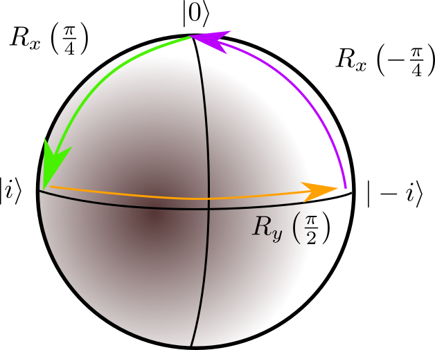 This shows the path taken on the Bloch sphere.
The qubit described with $|\psi\rangle = a |0\rangle + b|1\rangle$ resides in a three dimensional sphere embedded in four dimensions as the two complex numbers (each with two-degrees of freedom) are normalized so that $|a|^2 + |b|^2 = 1$.
However the Bloch sphere is two dimensional and embeded in three dimensions.
A position on it can be described with two angles, like latitude and longitude. To place the full qubit state onto the Bloch sphere a phase is discarded. This is a projection. The discarded global phase does not affect measurements of the qubit. However a series of transformations that take a point on the Bloch sphere along a loop back to its original point, may not bring the full state vector (including the global phase) back to its original state. The phase acquired is sometimes called geometric phase and is analogous to Berry's phase.