The Ising model is a model for ferromagnetism. The model consists of discrete variables that represent magnetic dipole moments of atomic spins that can be in one of two states (+1 or −1). The two-dimensional square-lattice Ising model is one of the simplest statistical models to show a phase transition.
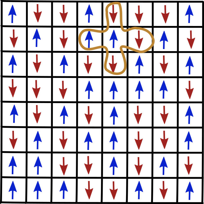
Above we show a square lattice with arrows representing each spin. Spins are either up or down. Nearest neighbors interact. Here in yellow I show the nearest neighbors of a single atom.
The energy is described with
$$ E = \sum_{a,b: ~nn} -J s_a s_b$$where $s_a, s_b$ are the spin values (either 1 or -1) at grid location $a$ and grid location $b$ where to specify a grid location you need to specify both $x$ and $y$ locations. The sum is assumed to only be over $a,b$ values that are nearest neighbors (as we have shown in yellow in the above figure), or two grid locations that are adjacent in the $x$ direction or adjacent in the $y$ direction.
To mimic a large area we can use periodic boundary conditions, so the left size of the square is adjacent to the right side and the top side is adjacent to the bottom side.
Magnetization
If the dipoles (spins) point in random directions then the overall magnetization is close to zero. But if they are preferentially aligned then the system has a macroscopic magnetic moment -- it is magnetized.
The magnetization is the average of all the spins! With $N$ the number of spins
$$M = \frac{1}{N}\sum_a s_a $$Energy when spins are the same
We repeat the equation for total energy
$$ E = \sum_{a,b: ~nn} -J s_a s_b$$
If coefficient $J$ (with units of energy) is positive then if two neighboring spins are the same then the contribution from the interaction lowers the energy.
This model has lowest possible energy state if all the spins are the same.
A positive $J$ and the negative sign in the energy expression give a model for ferromagnetism .
At low
temperature the system should magnetize and the spins should align.
Part 1
We start with two routines which are given below.
A routine that creates a 2d array and fills it with a random distribution of $\pm 1$.
A routine to calculate the total energy from a 2d array of spin values.
a. Write a routine that efficiently calculates the difference in energy if a single spin is flipped. The particular location where you flip the spin would be given by indices $i,j$. You should compute the energy different locally, using spin values at locations in the grid near $i,j$. (If you multiply whole arrays together the algorithm would be slower.)
b. Check that when you use your energy routine to calculate the energy difference that you get an answer that is consistent with that computed using the total energy routine, flipping the spin and then computing the total energy again.
c. Write a routine that calculates the magnetization.
import numpy as np

# example code! parts a,b done!

#create a 2dimensional Lx times Ly spin array and fill with random +-1 values
#does not need to be done efficiently with vectors because only called once
#creates and returns created spin array
#Lx and Ly should be the integer lengths of the 2x2 array
def fill_spin(Lx,Ly):
    spinarray = np.zeros((Lx,Ly))
    for i in range(0,Lx):
        for j in range(0,Ly):
            x = np.random.random()   #[0,1)
            if (x >= 0.5):
                spinarray[i,j] = 1
            else:
                spinarray[i,j] = -1

    return spinarray

# Compute total energy of spin array
# using a Hamiltonian H = sum_nn (- J s_a s_b)
#    nn = nearest neighbors (up down and right left)
# where spins are s_a, s_b
# inputs: spinarray, a 2d array of +1-1 spins
#   J is energy of spin interaction
# spinarray is a previously allocated 2darray
# nearest neighbors are 4 adjacent ones on a 2d grid
# using periodic boundary conditions for the 2d grid
# returns total summed energy
def energy(spinarray,J):
    center = spinarray
    up   = np.roll(spinarray,-1,axis=0)  # array shift up
    right= np.roll(spinarray,-1,axis=1)  # array shift right
    # nothing here depends on actual directions via symmetry
    sumt = np.sum((up + right)*center)
    # each nearest neighbor pair covered once
    # print(sumt) # for debugging
    E = -J*sumt # total energy
    return E
The Metropolis-Hastings algorithm
The Metropolis algorithm is the following Monte Carlo method.
Randomly select a grid position $i,j$ in two-dimensions. I found this routine usefull np.random.randint() to generate integer indices.
Compute the difference in energy if the spin of the atom at $i,j$ is flipped. If $E_1$ is the original energy and $E_2$ is the energy with that atom's spin flipped, then compute $$dE = E_2 - E_1$$
If $dE \le 0$ flip the spin at index $i,j$. The new configuration has lower energy.
If $dE>0$ then flip the spin at index $i,j$ using a probability $$ P = e^{-\beta dE}$$ with $\beta = 1/k_BT$ depending on temperature. The new configuration has higher energy. To do this you can randomly generate a number $x$ between $[0,1)$ and flip the spin at index $i,j$ if your randomly generated number $x < P$.
Repeat!
If the temperature is low, the system should become magnetized (all spins are in the same direction) and if the temperature is high the system should stay with magnetization near zero (spins are randomly oriented).
Part 2
- Write routines to implement iterations of the Metropolis algorithm.
A first routine, picks randomly a grid location and either flips or does not flip the spin at that location. The second routine calls the first routine $N_{it}$ times and stores the magnitization at each step.
- Setting $J=1$ and Boltzmann constant $k_B=1$, show that if temperature $T<1$ the system becomes magnetized.
If the grid is 50x50, you need to run at least $10^5$ steps. Plot magnetization as a function of time or iteration step including the steps where the spin flip was not accepted.
Show that if $T>3$ the system fluctuates around a magnetization near zero. The phase transition takes place at about $T\sim 2$ and you want to be above this temperature to see a non-magnetized state.
Show that two simulations that start at different magnetizations, converge to the same final magnetization.
For more information on the Ising model see https://en.wikipedia.org/wiki/Ising_model
To see the phase transition we could plot average magnetization (for many steps and after a relaxation period) as a function of temperature. At low temperature the system can either become magnetized with $M\to 1$ or $M\to -1$. When comparing results at different temperatures we might want to start with a slightly uneven spin distribution so that the grid always becomes magnetized in the same direction.
Checks to make sure your algorithm is working.
Check the sign of $dE$. If you have the wrong sign, the algorithm won't work.
Check that the entire 2d grid is covered in $i,j$. If you don't cover the entire grid, the simulation will not look right.
To make this routine efficient you do not want to compute the total energy each step. You only want to locally compute the change in energy $dE$ from a few positions in the array.
The time it takes the simulation to converge is of order a few times $N$ where $N$ is the number of spins. For a $50\times 50$ grid I found I needed to run 500000 steps at $k_BT = 0.6$. To check that you have run the routine long enough start at different levels of magnetization and make sure that the final magnetizations agree.