Problem set #4 PHY256 Problems with Solutions
Problem 1
Part 2.
$$\frac{dy}{dt} = y^2 + 1 $$It is useful to write $$ \frac{dy}{y^2 + 1 } = dt $$ A solution (which I can find without effort using https://www.wolframalpha.com/) $$ {\rm tan}^{-1} y = t + c $$ giving $$ y = {\rm tan} ( t + C)$$ where $C$ is a constant. Using the initial value of $y_0$ at $t=0$ $$C = {\rm arctan} y_0 $$
# solution for parts 1,3 with odeint
%pylab inline
import numpy as np
from scipy.integrate import odeint
from scipy.integrate import solve_ivp
import matplotlib.pyplot as plt
#from scipy.special import erfinv

# https://docs.scipy.org/doc/scipy/reference/generated/scipy.integrate.odeint.html

#initial condition
y0 = 0.03
# Set up time grid for integration
tmax=1.5;
dt = 0.001;
tt = np.linspace(0,tmax,200);  # the time vector

def func(y,t):  # equation for motion! this is dy/dt
    return y**2 + 1

def analytical_solution(y0,t):
    C = np.arctan(y0)
    return np.tan(t+C)

# solve the ordinary differential equation
yy=odeint(func,y0,tt,atol=1e-9)
# analytical solution
ysol = analytical_solution(y0,tt)
plt.plot(tt,yy,'ro')  # plot the ingegrated thing
plt.plot(tt,ysol,'b-')  # plot the analytical solution
plt.xlabel("time",fontsize=20)
plt.ylabel("y",fontsize=20)

#How well did it do?
print('error ' , ysol[-1]- yy[-1])  # compare the last times

Figure shows my prediction agrees with the integration.
# solution with solve_ivp which has completely different formats for everything!
# !#&#$@#$@#

#https://docs.scipy.org/doc/scipy/reference/generated/scipy.integrate.solve_ivp.html

def func2(t,y):  # equation for motion! this is dy/dt  note order flip in arguments!
    return y**2 + 1

def analytical_solution2(t,y0):  # I flipped the order here too
    C = np.arctan(y0)
    return np.tan(t+C)

tmax = np.max(tt)
# integrate
sol=solve_ivp(func2,[0,tmax],[y0],t_eval=tt,atol=1e-10) # arguments are not in the same order
# analytical solution
ysol = analytical_solution2(tt,y0)
plt.plot(sol.t,sol.y[0],'ro')  # plot the ingegrated thing
plt.plot(tt,ysol,'b-')  # plot the analytical solution
plt.xlabel("time",fontsize=20)
plt.ylabel("y",fontsize=20)

#How well did it do?
print('error ' , ysol[-1]- sol.y[0,-1])  # compare last points

- Rescaling
-
$$\frac{dz}{d\tau} = a+ bz^2 $$
Insert $z = \alpha y$, $\tau = \beta t$. $$ \frac{d \alpha y }{d \beta t} = a + b \alpha^2 y^2 $$ $$ \frac{dy}{dt} = \frac{\beta}{\alpha} \left(a + b \alpha^2 y^2 \right) $$ We set $$\frac{\beta}{\alpha} = \frac{1}{a} $$ and we get $$ \frac{dy}{dt} = 1 + \frac{b}{a} \alpha^2 y^2 $$ We now set $$ \frac{b}{a} \alpha^2 = 1$$ giving $$\alpha = \sqrt{ \frac{a}{b}}$$ and $$ \beta = \frac{\alpha}{a} = \sqrt{ \frac{1}{ab}} $$
Check units.
Assume that $z$ has units of length and $\tau$ has units of time.
Assume $y$ and $t$ are unitless.
$a$ is in units of length/time.
$b$ is in units of time$^{-1}$ length$^{-1}$.
$\beta$ must be in units of time.
$\alpha$ must be in units of length.
Using these units we check that $\alpha = \sqrt{a/b}$ is in units of $\sqrt{\frac{length/time}{length^{-1} time^{-1}}} = length$, as expected.
We check that $\beta = \sqrt{1/(ab)}$ is in units of $\sqrt{1 / (length/time \times time^{-1} length^{-1})} = time $, as expected.
Everything checks out.
Problem 2
# here is my qubit class for problem 2, 3
class qubit():
    def __init__(self,a,b):
        self.a =np.complex(a)  # make sure we have complex numbers
        self.b =np.complex(b)  # make sure is normalized
        self.normalize()

    def __repr__(self):
        return "qubit {}|0> + {}|1>".format(self.a,self.b)

    def __str__(self):
        return "qubit {:.2f}|0> + {:.2f}|1>".format(self.a,self.b)

    def normalize(self):
        length2 = self.a*np.conj(self.a) +  self.b*np.conj(self.b)
        self.a /= np.sqrt(length2)
        self.b /= np.sqrt(length2)

    # operate on the qubit with the Hadamard operator H
    def hadamard(self):
        anew = (self.a + self.b)/np.sqrt(2)
        bnew = (self.a - self.b)/np.sqrt(2)
        self.a = anew
        self.b = bnew

    # operate on the qubit with the Pauli spin matrix sigma_x
    def sigma_x(self):
        anew = self.b
        bnew = self.a
        self.a = anew
        self.b = bnew

    # operate on the qubit with the Pauli spin matrix sigma_y
    def sigma_y(self):
        anew = -1j*self.b
        bnew =  1j*self.a
        self.a = anew
        self.b = bnew


    # operate on the qubit with the Pauli spin matrix sigma_z
    def sigma_z(self):
        anew =  1*self.a
        bnew = -1*self.b
        self.a = anew
        self.b = bnew

    # return probability of measuring spin up
    def prob_up(self):
        return np.real(self.a * np.conj(self.a) )   # return a real number

    # simulate a measurement of spin
    def measure_spin(self):
        p_up = self.prob_up()
        r = random.random()
        if (r < p_up):
            self.a = self.a / np.abs(self.a)  # spin up measured
            self.b =0
            return 1
        else:
            self.b = self.b / np.abs(self.b)  # spin down measured
            self.a =0
            return 0

    # exponential of Pauli matrix sigma_x and with angle alpha
    def R_x(self,alpha):
        anew =    np.cos(alpha)*self.a + 1j*np.sin(alpha)*self.b
        bnew = 1j*np.sin(alpha)*self.a +    np.cos(alpha)*self.b
        self.a = anew
        self.b = bnew

    # exponential of Pauli matrix sigma_y
    def R_y(self,alpha):
        anew =    np.cos(alpha)*self.a + np.sin(alpha)*self.b
        bnew = -1*np.sin(alpha)*self.a + np.cos(alpha)*self.b
        self.a = anew
        self.b = bnew

    # exponential of Pauli matrix sigma_z
    def R_z(self,alpha):
        anew =    np.cos(alpha)*self.a + 1j*np.sin(alpha)*self.a
        bnew =    np.cos(alpha)*self.b - 1j*np.sin(alpha)*self.b
        self.a = anew
        self.b = bnew
q0 = qubit(1.0+0j,0+1j)
q0
print(q0)
q0.hadamard()
print(q0)
print(q0.measure_spin())
print(q0)
for i in range(10):
    q0 = qubit(1.0+0j,0+1j)
    print(q0.measure_spin())
q0 = qubit(1.0+0j,0+1j)
q0.prob_up()
Problem 3
q0 = qubit(1.0,0)
print(q0)
q0.R_x(np.pi/4)  # gives |i> on equator
print(q0)
q0.R_y(np.pi/2)   # rotates along equator to opposite side
print(q0)
q0.R_x(-np.pi/4)   # now go back to pole
print(q0)
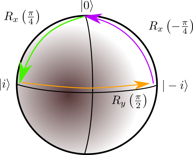
The qubit described with $|\psi\rangle> = a |0\rangle + b|1\rangle$ resides in a three dimensional sphere embedded in four dimensions as the two complex numbers (each with two-degrees of freedom) are normalized so that $|a|^2 + |b|^2 = 1$.
However the Bloch sphere is two dimensional and embeded in three dimensions.
A position on it can be described with two angles, like latitude and longitude.
To place the full qubit state onto the Bloch sphere a phase is discarded. This can be
considered a projection.
The discarded phase
does not affect measurements of the qubit. However a series of transformations that take
a point on the Bloch sphere along a loop back to its original point, may not
bring the full state vector (including the extra phase) back to its original state.
The phase acquired is sometimes called geometric phase and is analogous to
Berry's phase.