Problem Set 10. Quantum Computing with QuTiP
%matplotlib inline
from IPython.display import Image
from qutip import *    # here is where we import QuTiP
from qutip.qip.operations import cnot   # CNOT op
from qutip.qip.operations import snot   # Hadamard op
from qutip.qip.circuit import QubitCircuit
import numpy as np
We are using the QuTiP package which is a Quantum Toolbox in Python, see http://qutip.org/
You will need to install QuTiP to do this assignment
you may need to do this: conda config --add channels conda-forge
before you conda install qutip
Alternatively you can
pip install qutip
For information on quantum gates see http://en.wikipedia.org/wiki/Quantum_gate
Basic operations in QuTiP http://qutip.org/docs/latest/guide/guide-basics.html?highlight=multiply
Tensor products in QuTiP http://qutip.org/docs/latest/guide/guide-tensor.html
For a tutorial using QuTiP to apply quantum gates https://nbviewer.jupyter.org/github/qutip/qutip-notebooks/blob/master/examples/quantum-gates.ipynb
Problem 1. The Deutsch black box problem
We have an unknown function $f(x)$ that takes either 0 or 1 and returns 0 or 1. There are 4 possibilities for this function $$f(x) = 0 \qquad f(x) = 1 \qquad f(x) =x \qquad f(x) = {\rm NOT}\ x $$ The left two possibilities are constant and the right two are balanced.
We want to determine if $f(x)$ is constant or balanced and with a single measurement and a single query. This is impossible with a classical computer but is possible with a quantum computer.
Implement the Deutsch algorithm as shown in this figure as a quantum circuit with 2 qubits.
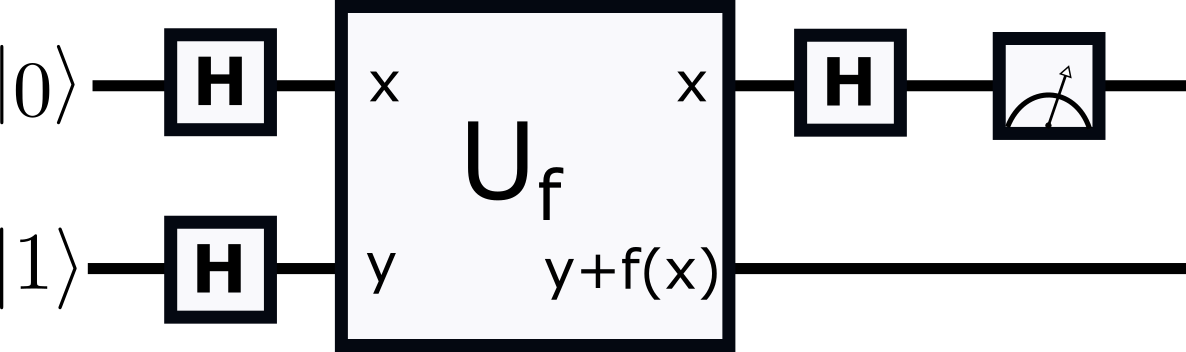
The Figure represents a series of operations on an initial state $$ ({\bf H} \otimes {\bf I} ) * {\bf U}_f * ({\bf H} \otimes {\bf H}) |01\rangle$$
Note that operations are left to right in the figure but right to left in the equation above.
You create the state $|01\rangle$. The $\bf H$ are Hadarmard operators and ${\bf U}_f$ is an operator in the 2 qubit space that depends on the function $f()$.
You operate on the state with ${\bf H} \otimes {\bf H}$. You operate on the resulting state with $U_f$. Then you operate on the resulting state with ${\bf H} \otimes {\bf I}$. Then you measure the first qubit (top in figure). The algorithm determines whether the function is balanced or constant from the measurement.
$U_f$ takes $|x,y\rangle \to |x, y + f(x)\rangle$. $U_f$ does this \begin{align} |00\rangle &\to |0,0+f(0)\rangle = |0,f(0)\rangle \\ |01\rangle &\to |0,1+f(0)\rangle = |0,NOT \ f(0)\rangle \\ |10\rangle &\to |0,0+f(1)\rangle = |1, f(1)\rangle \\ |11\rangle &\to |0,1+f(1)\rangle = |1, NOT\ f(1)\rangle \end{align}
If $f(x)=0$, $U_f$ is the identity.
If $f(x)=1$, $U_f$ flips the second qubit; $$U_f = I \otimes \sigma_x$$
If $f(x) = x$, then $U_f$ only flips the second qubit if the first qubit is This is a CNOT (a controlled NOT) with control the first bit and target the second bit $$U_f = {\rm CNOT(control=0,target=1)}$$
If $f(x) = {\rm NOT} \ x$ then $U_f$ flips the second qubit if the first qubit is 0. This is a CNOT with target the second bit but with control the NOT of the first bit.
$$U_f = {\rm CNOT(control=0,target=1)} * ( \sigma_x \otimes I) $$
I have written a routine below that gives you $U_f$.
a. Write a routine that simulates the circuit with a series of quantum operators applied to an initial state. You want to be able to do this four times, once for each type of function $f()$. Take a look at the function $U_f$ below and consider passing a string to your routine allowing you to choose the black box function $f()$. Your circuit should create the ket $|01\rangle$ and tensor operators for the Hadamard operations. Your routine should apply the operators in the quantum circuit to the ket. Then your routine should return the probability that the first qubit in the final state is 0.
b. Show that, after applying the quantum circuit, measurement of the first qubit always gives 0 with 100\% probability if the function $f(x)$ is constant and gives 1 with 100\% probability if the function is balanced.
# used in problem 1
# this is the black box or oracle
# Return a quantum operator on 2 qubits that returns the operation $U_f$.
# the unitary operator should give |x,y> \to |x, y+ f(x)> where + is mod 2
# the operator depends on the function type
# f_type is a string
#        '0' for f(x)=0
#        '1' for f(x)=1
#        'x' for f(x)=x
#        'N' for f(x) = NOT x
def U_f(f_type):
    if (f_type=='0'): # f(x)=0
        return tensor(qeye(2),qeye(2)) # identity transformation,
        # using a tensor product otherwise can't be combind easily with other operators
    if (f_type=='1'): # f(x)=1
        return tensor(qeye(2),sigmax()) # second qubit is flipped
    if (f_type=='x'): # f(x)=x
        return cnot(2,control=0,target=1)
    if (f_type=='N'): # f(x)=NOT x
        return cnot(2,control=0,target=1)*tensor(qeye(2),sigmax())
    return tensor(qeye(2),qeye(2))  #return identity if not a known f_type

print(U_f('1') )  # quick test! to see if the function works
print(U_f('x') )
print(U_f('N') )
Problem 2. A quantum random walk
A Quantum random walk, as introduced by Aharonov, Davidovich, and Zagury 1993, is a sequence of unitary transformations. They can also be called quantum cellular automata. Unlike a classical and stochastic random walk, all transformations are unitary and hence reversible. The walk does not lose its recollection of the initial state and it cannot converge to a stationary distribution.
see https://en.wikipedia.org/wiki/Quantum_walk
We explore a discrete quantum random walk of a spin on a circle.
Take a state space that is a tensor product of a space with two states (a qubit),
${\cal H}_2$,
and a space with $N$ states, ${\cal H}_N$.
A basis for this space is
$$|j n\rangle$$
where $j \in \{0,1\}$ is spin up or down and $n \in \{0,N-1\}$. The $N$ dimensionsal Hilbert space can be described as $N$ possible particle positions.
The entire Hilbert space is a tensor product space ${\cal H} = {\cal H}_2 \otimes { \cal H}_N$.
We start with $|\psi\rangle = |00\rangle$ and alternate applying a spin mixing operator $${\bf H} \otimes {\bf I}$$ and a position change that depends on the spin $${\bf C} \equiv {\bf P}_0 \otimes {\bf U}_+ + {\bf P}_1 \otimes {\bf U}_-$$
${\bf H}$ is the Hadamard operator on the spin state (in ${\cal H}_2$) and it takes \begin{align} {\bf H}|0\rangle &= \frac{1}{\sqrt{2}} ( |0\rangle + |1\rangle )\\ {\bf H}|1\rangle &= \frac{1}{\sqrt{2}} ( |0\rangle - |1\rangle ) \end{align} $$ {\bf H} = \frac{1}{\sqrt{2}}\left( \begin{array} {cr} 1 & 1 \\ 1 & -1 \end{array} \right) $$ The transformation ${\bf H} \otimes {\bf I}$ shifts the spin state but operates on a state in $\cal H$.
${\bf P}_0$ projects the spin state onto $|0\rangle$ and ${\bf P}_1$ projects the spin state onto $|1\rangle$, \begin{align} {\bf P}_0|0\rangle &= |0\rangle \\ {\bf P}_0|1\rangle &= 0 \\ {\bf P}_1|0\rangle &= 0 \\ {\bf P}_1|1\rangle &= |1\rangle \end{align} These two operate on spin states, or those in ${\cal H}_2$. We can also write \begin{align} P_0 &= |0\rangle \langle 0| = \left(\begin{array}{cc} 1 & 0 \\ 0 & 0 \end{array} \right) \\ P_1 &= |1\rangle \langle 1| = \left(\begin{array}{cc} 0 & 0 \\ 0 & 1 \end{array} \right) \end{align}
The operators ${\bf U}_+$ and ${\bf U}_-$ raise and lower $n$ \begin{align} {\bf U}_+ |n\rangle & = |n+1\ {\rm mod}\ N\rangle \\ {\bf U}_- |n\rangle & = |n-1\ {\rm mod}\ N\rangle \end{align} These two operate on states in ${\cal H}_N$. We can also write \begin{align} {\bf U}_+ &= \sum_{j=0}^{N-2} |j+1\rangle \langle j| + |0 \rangle \langle N-1 | = \left( \begin{array}{ccccccc} 0 & 0 & 0 & 0 & .. & 0 & 1 \\ 1 & 0 & 0 & 0 & .. & 0 & 0 \\ 0 & 1 & 0 & 0 & .. & 0 & 0 \\ 0 & 0 & 1 & 0 & .. & 0 & 0 \\ 0 & 0 & 0 & 1 & .. & 0 & 0 \\ : & : & : & : & : & : & :\\ 0 & 0 & 0 & 0 & .. & 1 & 0\\ \end{array} \right) \\ {\bf U}_- &= \sum_{j=1}^{N-1} |j-1\rangle \langle j| + | N-1 \rangle \langle 0 | =\left( \begin{array}{ccccccc} 0 & 1 & 0 & 0 & .. & 0 &0 \\ 0 & 0 & 1 & 0 & .. & 0 &0 \\ 0 & 0 & 0 & 1 & .. & 0 &0 \\ : & : & : & : & : & : & : \\ 0 & 0 & 0 & 0 & .. & 0& 1\\ 1 & 0 & 0 & 0 & .. & 0& 0\\ \end{array} \right) \end{align}
The operator ${\bf C}$ moves the particle to the right if the spin is up and moves the particle to left if the spin is down. This is why the procedure can be called a random walk. Because ${\bf U}_+ |N-1\rangle = |0\rangle$ and ${\bf U}_- |0 \rangle = |N-1\rangle$, the end of the $N$ state space is connected with the beginning of it, so our position space is equivalent to $N$ equidistant points on a circle.
We can think of operator $\bf C$ as defining a network of connections between states in the N-dimensional Hilbert space ${\cal H}_N$. The $\bf C$ operater entangles the spin with the particle position.
a. Below I have written a routine that returns ${\bf U}_+$. This returns a quantum operator in the $N$ dimensional Hilbert space. Write a similar routine that returns ${\bf U}_-$. Check that it is unitary. Unitary matrices satisfy $U U^\dagger = {\bf I}$. I have written a routine to check unitarity and you can use this. Or you could instead compute $U U^\dagger$ and look at it to make sure that it is an identity matrix.
b. Below I have written a routine that returns projection operator ${\bf P}_0$.
Write a similar
routine that returns ${\bf P}_1$. These are operators in the 2 dimensional Hilbert space.
Chose an $N$ integer value for the number of possible positions. Start with something small and then later you can increase to something bigger like 50 or 100.
c. Construct the operator ${\bf H} \otimes {\bf I}$ using the qutip routine tensor().
d. Construct the operator ${\bf C}$. Check that it is unitary.
e. Combine these two into a single operator $$ {\bf V} = ({\bf H} \otimes {\bf I} ) *{\bf C}$$
e. Create an initial state $| 0\frac{N}{2}\rangle$ with
psi0 = tensor(ket('0'),fock(N,int(N/2)))
or an initial state $|00\rangle$ with
psi0 = tensor(ket('0'),fock(N,0))
The routine will work equal well with either but your plots might look better starting with $| 0\frac{N}{2}\rangle$.
f. Write a loop that applies the operator $\bf V$ over and over again to your statevector.
Each time print out or plot the probabilities to be in each of the states in the N-dimensional Hilbert space. I have written for you a routine
prob_N() to help you do this.
The probabilities (of being in state $|n\rangle $) should go up and down (even states are effected differently than odd states) and the distribution should rapidly spread out from the initial state as you iterate!
# This routine checks if a quantum operator U is unitary
# helper routine for problem 3
# returns 0 if not unitary, returns 1 if unitary
small = 1e-6  # sometimes matrices are not exact integers,
# this sets how close we want to check the difference
def check_unitary(U):
    if (U.type != 'oper'):
        return 0  # is not an operator
    z = U*U.dag()  # should be the identity matrix if unitary
    matrix = z.data   # should be the identity matrix if unitary
    #print(matrix)
    dim = U.shape[0]  # assumes is a square matrix
    # check every matrix value to make sure it looks like the identity matrix
    for i in range(0,dim):
        for j in range(0,dim):
            matrixvalue = matrix[i,j]
            if (i!=j):
                if (abs(matrixvalue) > small):  # has something other than 0 off diagonal
                    return 0  # is not unitary
            else:  # checking the diagonal entries
                if (abs(matrixvalue-1) > small):  # has something other than 1 on diagonal
                    return 0  # is not unitary
    # if you get to here z looks like the identity matrix and so U is unitary
    print('U is unitary')
    return 1 # is unitary!

# some tests of this routine
print(check_unitary(cnot()))
#print(check_unitary(P0))

# helper routine for problem 3
# given a state psi in product Hilbert space H_2 otimes H_N
# return a vector of probabilities
# to be in each of the |n> states
# psi is a vector in the product Hilbert space psi is a sum of basis vectors |jn>
#   where |j> is a spin and |n> is in an N dimensional Hilbert space
def prob_N(N,psi):
    nprobs= np.zeros(N)  # allocate a vector of N values
    for i in range(0,N):
        nproj=projection(N,i,i)    # projection operator for state |i>
        # the first argument is the dimension of the Hilbert space
        v = tensor(qeye(2),nproj)  # to take into account both spin possible values
        nprobs[i] = expect(v,psi)  # probability of being in |n>
    return nprobs  # return the vector of probabilities


# tests of the routine prob_N
N=4
ss = (ket('0') + ket('1')).unit()
psi0 = tensor(ss,fock(N,2))
psi1 = tensor(ss,fock(N,3))
psi = (psi0 + psi1).unit()
print(prob_N(N,psi))  #looks good!
# return an operator that does |n> \to |n+1 mod N>
def make_Uplus(N):
    U = projection(N,0,N-1)  # this gives a matrix with a single 1 in it
    # the first argument is the dimension of the Hilbert space
    # the second two arguments are i,j giving |i><j|
    for i in range(0,N-1):
        U = U + projection(N,i+1,i)
    #print(U)
    return U

# test
print(make_Uplus(7))

# projection operator for problem 2
P0= projection(2,0,0)  # this projects to |0>
# this is equal to |0><0|
print(P0)
from qutip.ipynbtools import version_table
version_table()
about()